Poisson Equation
\[\begin{split}\begin{cases}
-\nabla^2 u = f(x) &\text{ in } \Omega \\
u = 0 & \text{ on } \partial\Omega
\end{cases}\end{split}\]
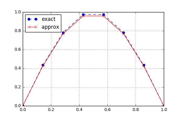
1 Dimensional Case
- Example
>>> import numpy as np
>>> from mozart.mesh.rectangle import interval
>>> from mozart.poisson.fem.interval import solve
>>> f = lambda x: np.pi ** 2 * np.sin(np.pi * x)
>>> u_D = lambda x: np.zeros_like(x)
>>> nrElems, degree = (7, 1)
>>> c4n, n4e, n4db, ind4e = interval(0, 1, nrElems, degree)
>>> u = solve(c4n, n4e, n4db, ind4e, f, u_D, degree)
>>> u
array([ 0.        ,  0.42667492,  0.76884164,  0.95872984,  0.95872984,
0.76884164,  0.42667492,  0.        ])
-
mozart.poisson.fem.interval.computeError(c4n, n4e, ind4e, exact_u, exact_ux, approx_u, degree, degree_i)[source]¶ Computes L^2-error and semi H^1-error between exact solution and approximate solution.
- Parameters
c4n(float64 array) : coordinates for nodesn4e(int32 array) : nodes for elementsind4e(int32 array) : indices for elementsexact_u(lambda) : exact solutionexact_ux(lambda) : derivative of exact solutionapprox_u(float64 array) : approximate solutiondegree(int32) : Polynomial degreedegree_i(int32) : Polynomial degree for interpolation
- Returns
L2error(float64) : L^2 error between exact solution and approximate solution.sH1error(float64) : semi H^1 error between exact solution and approximate solution.
- Example
>>> N = 2
>>> from mozart.mesh.interval import interval
>>> c4n, n4e, n4db, ind4e = interval(0, 1, 4, 2)
>>> f = lambda x: np.pi ** 2 * np.sin(np.pi * x)
>>> u_D = lambda x: np.zeros_like(x)
>>> from mozart.poisson.fem.interval import solve_p
>>> x = solve_p(c4n, n4e, n4db, ind4e, f, u_D, N)
>>> from mozart.poisson.fem.interval import computeError
>>> exact_u = lambda x: np.sin(np.pi * x)
>>> exact_ux = lambda x: np.pi * np.cos(np.pi * x)
>>> L2error, sH1error = computeError(c4n, n4e, ind4e, exact_u, exact_ux, x, N, N+3)
>>> L2error
0.0020225729623142077
>>> sH1error
0.05062779815975444
-
mozart.poisson.fem.interval.getMatrix(degree)[source]¶ Get FEM matrices on the reference domain I = [-1, 1]
- Paramters
degree(int32) : degree of polynomial
- Returns
M_R(float64 array) : Mass matrix on the reference domainS_R(float64 array) : Stiffness matrix on the reference domainD_R(float64 array) : Differentiation matrix on the reference domain
-
mozart.poisson.fem.interval.solve(c4n, n4e, n4db, ind4e, f, u_D, degree)[source]¶ Computes the coordinates of nodes and elements.
- Parameters
c4n(float64 array) : coordinates for nodesn4e(int32 array) : nodes for elementsn4db(int32 array) : nodes for Dirichlet boundaryind4e(int32 array) : indices for elementsf(lambda) : source termu_D(lambda) : Dirichlet boundary conditiondegree(int32) : Polynomial degree
- Returns
x(float64 array) : solution
- Example
>>> N = 2
>>> from mozart.mesh.interval import interval
>>> c4n, n4e, n4db, ind4e = interval(0, 1, 4, 2)
>>> f = lambda x: np.ones_like(x)
>>> u_D = lambda x: np.zeros_like(x)
>>> from mozart.poisson.fem.interval import solve
>>> x = solve(c4n, n4e, n4db, ind4e, f, u_D, N)
>>> x
array([ 0.       ,  0.0546875,  0.09375  ,  0.1171875,  0.125    ,
   0.1171875,  0.09375  ,  0.0546875,  0.       ])